Analysis Tutorial 1: Basic Analysis and Templates 1

This tutorial showcases some of the basic functionality of EMDtool, including

* Creating a motor model from templates
* Running time-static analysis and post-processing basic results

Setting dimensions
Creating rotor geometry.
Creating stator geometry.
Meshing the geometry
Creating a Model
Setting supply
Running analysis
Plotting results

Setting dimensions

First, let us set the dimensions required. For simplicity, we begin by initializing an empty structure.

Finally, let us initialize a timer to see how long stuff actually takes:

tic;
addpath(genpath('../EMDtool'));
dim = struct();

Next, let's set some general dimensions and specs.

%general dimensions
dim.p = 10; %number of pole-paits
dim.Qs = 24; %number of stator slots
dim.delta = 1e-3; %total effective airgap
dim.leff = 70e-3; %core length

dim.temperature_rotor = 100;
dim.temperature_stator = 120;

Then, let us define our winding.

%winding parameters
winding = ConcentratedWindingSpec(dim);
winding.N_layers = 2;
winding.filling_factor = 0.5;
winding.N_series = 12;

dim.stator_winding = winding;
dim.symmetry_sectors = dim.stator_winding.symmetry_period();

Furthermore, let us set some general dimensions. These help the templates to determine whether we are making an inrunner or an outrunner motor.

dim.Rout = 50e-3; %airgap-side radius of rotor
dim.Sin = dim.Rout - dim.delta; %airgap-side radius of stator
dim.Sout = 28e-3; %frame-side radius of stator

Finally, let's specify the materials used. For the default materials available, check out here.

dim.magnet_material = 14; %Magnet material
dim.rotor_core_material = 4; %rotor iron material
dim.stator_core_material = 4; %stator core material
dim.stator_wedge_material = 0; %air; no wedge

Creating rotor geometry.

Now, let's set some more dimensions.

%rotor dimensions
dim.hyr = 5e-3; %rotor yoke thickness
dim.h_sleeve = 0e-3; %no retaining sleeve for PMs
dim.hpm = 3e-3; %PM thickness
dim.alpha_pm = 0.8; %PM pitch, relative to pole pitch
dim.is_halbach = false; %no Halbach array

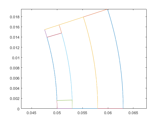
...and create and plot the geometry:

rotor = SPM1(dim);

figure(1); clf; hold on; box on; axis equal;
rotor.plot_geometry();
snapnow;

Creating stator geometry.

Next, let's do the same for the stator. There are oly a few more dimensions to set.

%stator dimensions
dim.htt_s = 1e-3; %tooth tip height
dim.htt_taper_s = 0.5e-3;
dim.hslot_s = 14e-3; %total slot depth, airgap to bottom
dim.wtooth_s = 5e-3; %tooth width
dim.wso_s = 2e-3; %slot opening width
dim.r_slotbottom_s = 1e-3; %slot bottom fillet radius

dim.stator_stacking_factor = 0.99;

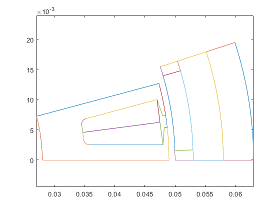
Create the geometry, and plot it.

stator = Stator(dim);

figure(1);
stator.plot_geometry();
snapnow;

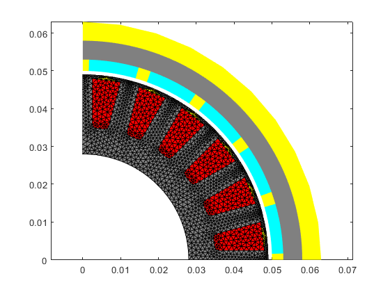
Meshing the geometry

Pretty self-evident, huh?

stator.mesh_geometry();
rotor.mesh_geometry();

figure(2); clf; hold on; box on; axis equal;
stator.visualize('linestyle', '-');
rotor.visualize();
snapnow;
toc

Elapsed time is 2.129119 seconds.

Creating a Model

Now, we create a model, an object for encapsulating all the relevant components, aspects, and behaviour of our design. Since we are dealing with a rather standard radial-flux motor, the base class RFmodel will do.

tic;
motor = RFmodel(dim, stator, rotor);

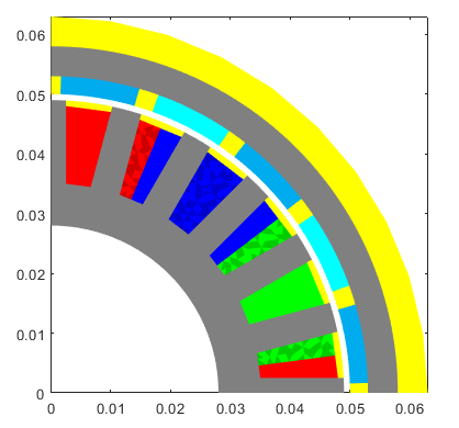
For reasons, let's also visualize the model to see e.g. the winding layout highlighted with different colours.

figure(2); clf; hold on; box on; axis equal;
motor.visualize();
snapnow;

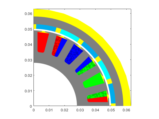
Let's also create a MagneticsProblem object for representing the problem we're analysing.

problem = MagneticsProblem(motor);
toc;

Elapsed time is 0.377287 seconds.

Setting supply

For now, we're going to be using a current supply model, meaning we're not taking induced voltages etc. into account.

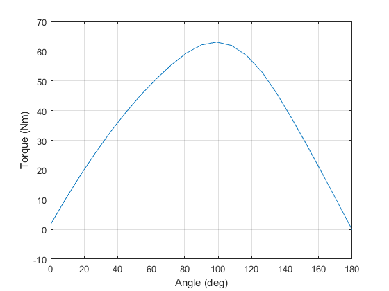
Let's run a sweep of load angles from 0 to 180 degrees, to compute a rough torque curve. First, create an array for the load angles

tic;
load_angles = linspace(0, pi, 21); %load angles to analyse

Then, do an inverse Park-Clarke transformation to get the instantaneous phase currents from the dq-components:

Is = xy(80*[cos(load_angles); sin(load_angles)], problem)

Is =

  Columns 1 through 7

   77.2741   73.0836   67.0936   59.4516   50.3456   40.0000   28.6694
  -20.7055   -8.3623    4.1869   16.6329   28.6694   40.0000   50.3456
  -56.5685  -64.7214  -71.2805  -76.0845  -79.0151  -80.0000  -79.0151

  Columns 8 through 14

   16.6329    4.1869   -8.3623  -20.7055  -32.5389  -43.5711  -53.5304
   59.4516   67.0936   73.0836   77.2741   79.5618   79.8904   78.2518
  -76.0845  -71.2805  -64.7214  -56.5685  -47.0228  -36.3192  -24.7214

  Columns 15 through 21

  -62.1717  -69.2820  -74.6864  -78.2518  -79.8904  -79.5618  -77.2741
   74.6864   69.2820   62.1717   53.5304   43.5711   32.5389   20.7055
  -12.5148    0.0000   12.5148   24.7214   36.3192   47.0228   56.5685

Set the current array as source current...

C = motor.circuits.get('Phase winding');
C.set_source('uniform coil current', Is);

Running analysis

...and solve a series of static problems.

pars = SimulationParameters('rotorAngle', 0*load_angles/dim.p, 'silent', true);
solution = problem.solve_static(pars);

Plotting results

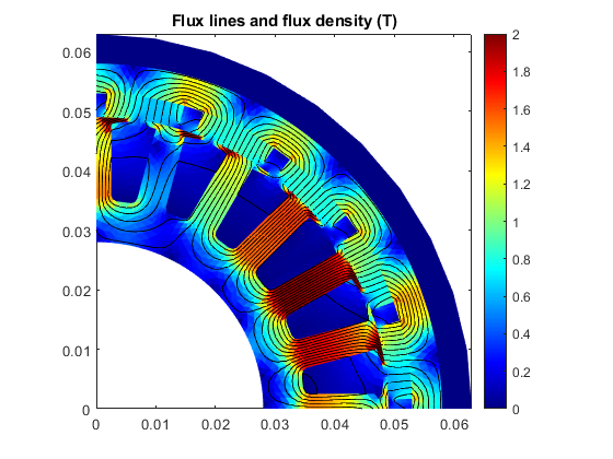
Finally, plot the torque curve and the flux density at peak torque.

T = motor.compute_torque(solution);
figure(6); clf; hold on; box on; grid on;
plot(load_angles/pi*180, T);
xlabel('Angle (deg)');
ylabel('Torque (Nm)');
snapnow
toc

figure(7); clf; hold on; box on;
motor.plot_flux( solution, 11);

Elapsed time is 1.751505 seconds.

(Back to index)