Geometry Tutorial 1: Meshing a rectange

This simple tutorial will demonstrate how to build and mesh simple geometries from scratch.

Contents

Create and mesh a rectangle

Create the corner Points.

p1 = Point([0,0], 0.3);
p2 = Point([1,0], 0.3);
p3 = Point([1,1], 0.3);
p4 = Point([0,1], 0.3);

Each Point consists of its coordinates, plus it characteristic length. The latter is a number, representing the maximum edge length near the point, in the final meshed geometry.

Next, create a Surface object and visualize it.

s = Surface('rectangle'); %create empty object
s.add_curve(geo.line, p1, p2); %add first boundary segment
s.add_curve(geo.line, p2, p3); %ditto for the remaining 3
s.add_curve(geo.line, p3, p4);
s.add_curve(geo.line, p4, p1);

clf; axis equal;
s.plot('ko-'); %visualize surface
axis([-0.5 1.5 -0.5 1.5]); %loosen axes to see properly.

Next, mesh the geometry using the gw (gmsh wrapper) class.

g = gw(s); %initialize the object with the surface

[nodes, elements, surfaces] = g.mesh(); %creating and loading mesh

Warning: No periodic lines were detected. Please verify that this is appropriate
for the geometry 

For reference, let's plot the resulting mesh.

clf; axis equal;
triplot(elements', nodes(1,:), nodes(2,:))

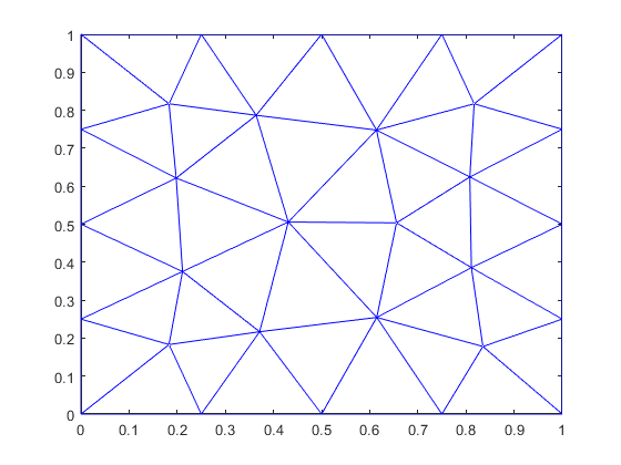
Here, nodes and elements contain the coordinates of the mesh nodes (as doubles), and the element definitions (as integer indices of the corresponding nodes), respectively:

nodes(:, 1:5)
elements(:, 1:5)

ans =

         0    1.0000    1.0000         0    0.7500
    1.0000         0    1.0000         0    1.0000


ans =

    19    17    22    24    22
    22    22    19    22    18
    23    24    26    26    23

Create and mesh a more complex geometry

This time, let's try some more advanced functionality:

Let's begin. Our new geometry will again be a rectangle, with a triangular hole near the bottom-left corner. For that purpose, let us redefine our first point to have a smaller characteristic length. This will force the resulting mesh to be denser around this region.

p1 = Point([0,0], 0.1);

Next, let's redefine our surface. While we're at it, let's demonstrate chaining several segment definitions together.

s = Surface('rectangle', ...
    geo.line, p1, p2, ...
    geo.line, p2, p3, 'right_boundary', ...
    geo.line, p3, p4, ...
    geo.line, p4, p1);

Additionally, as you can see the line Curve joining p2 and p3 has now been given the name 'right_boundary'.

Next, let's add a hole inside the geometry. We begin by defining three additional points:

ph1 = Point([0.2, 0.2], 0.05);
ph2 = Point([0.4, 0.2], 0.05);
ph3 = Point([0.2, 0.4], 0.05);

Then, we define the would-be hole with these points. The hole is a Surface with two straight boundaries plus one curved:

hole = Surface('hole'); %so-far empty
hole.add_curve(geo.line, ph1, ph2); %straight line
hole.add_curve(geo.arc, ph2, ph1, ph3); %an arc joining ph2 and ph3, centered at ph1
hole.add_curve(geo.line, ph3, ph1);

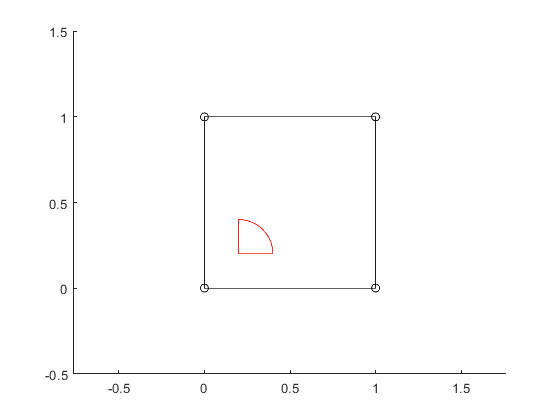
Now, let's visualize both together.

clf; axis([-0.5 1.5 -0.5 1.5]); axis equal;
s.plot('ko-'); %visualize surface
hole.plot('r-');

Now, add the hole to the larger surface:

s.add_curve(geo.hole, hole);

Next, the geometry is again meshed.

g = gw(s, hole); %initialize the object with the surface

[nodes, elements, surfaces] = g.mesh(); %creating and loading mesh

Warning: No periodic lines were detected. Please verify that this is appropriate
for the geometry 

As can be seen, the surfaces object now contains both the surfaces and the named line:

surfaces.keys()

ans =

  3×1 cell array

    {'right_boundary'}
    {'rectangle'     }
    {'hole'          }

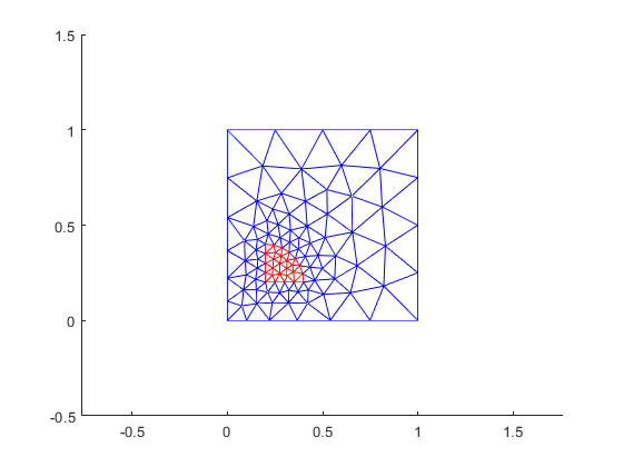
Finally, let's visualize the mesh.

clf; hold on; axis([-0.5 1.5 -0.5 1.5]); axis equal;
triplot(elements(:, surfaces.get('rectangle'))', nodes(1,:), nodes(2,:), 'b')
triplot(elements(:, surfaces.get('hole'))', nodes(1,:), nodes(2,:), 'r')

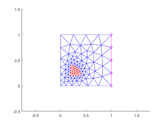
To plot the boundary nodes, we note that they are actually defined by the boundary edges

bnd_edges = surfaces.get('right_boundary')

plot( [nodes(1, bnd_edges(1,:)); nodes(1, bnd_edges(2,:))], ...
    [nodes(2, bnd_edges(1,:)); nodes(2, bnd_edges(2,:))], 'md-');

bnd_edges =

     6    33    34    35
    33    34    35     7

What to do next

By now, you should have an idea of how the EMDtool toolbox handles geometries. Next, you'll create a simple geometry template for a switched reluctance motor, and how to fully utilize the toolbox functionality to make your model creation workflow as simple as possible.

But, while you're here, please take a second to fill this form. You'll help to develop the toolbox further, and can opt in to receive updates of its progress.

All done? Great - you can now head on to the Advanced Example.

(Back to index)

Published with MATLAB® R2020a