Geometry Tutorial 2: (Almost) Creating a Rotor Template

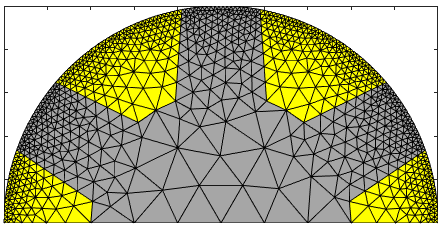
In this tutorial, you will almost learn how to create a geometry template for the rotor of a simple switched reluctance motor (SRM). (Indeed, the geometry will be fully usable, just not encapsulated inside its own Matlab class).

Along the journey, we will also learn some other useful items:

Handy methods of the Point class.
Utilizing the geometry base class GeoBase and its subclasses to simplify many meshing steps.

Initializing dimensions
Creating the tooth tip
Creating the tooth body and rotor core
Creating a Geometry object
Meshing the geometry object
Adding polegap domains
A Closer look at GeoBase
What to read next?

Initializing dimensions

We begin by collecting the important dimensions inside a Matlab struct. Why? This allows us to collect all rotor-related dimensions under a single Matlab variable. Furthermore, turning this script into a function later is then much easier.

Now, let's skip to the business and set some dimensions:

dimensions = struct();
dimensions.Rout = 50e-3; %outer diameter of our rotor
dimensions.Qr = 6; %number of rotor teeth
dimensions.w_tooth_r_out = 18e-3; %tooth tip width
dimensions.w_tooth_r_in = 21e-3; %tooth width near rotor yoke
dimensions.h_tooth_r = 20e-3; %tooth height

As can be seen, our simple rotor geometry is fully determined by only a few dimensions:

Its outer radius (or diameter, whichever you prefer)
Number of poles
The height of the rotor tooth, and its width at the top and bottom

Creating the tooth tip

We begin by creating the tip of the rotor tooth. First, let us assume we have a single rotor tooth laying centered on the x-axis. Next, we create a Point to represented the counter-clockwise corner of the tooth tip:

pout_clockwise = Point([sqrt(dimensions.Rout^2-(dimensions.w_tooth_r_out/2)^2), ...
    -dimensions.w_tooth_r_out/2], 1e-3);

Note how the x-coordinate of the Point is not exactly dimensions.Rout. Instead, it's somewhat smaller according to the Pythagorean theorem to maintain the correct airgap radius:

norm(pout_clockwise) - dimensions.Rout

ans =

     0

However, the recommended way of creating rotor pole shapes for EMDtool is not to have the pole d-axis centered along the x-axis.

Instead, the geometry should be rotated by one half of the pole pitch.

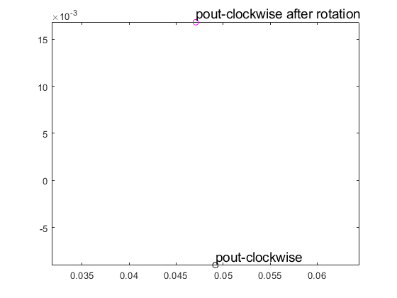
Let us do that now for the point we just created, and plot it before and after the rotation:

figure(1); clf; hold on;  box on; axis equal;
pout_clockwise.plot('pout-clockwise', 'ko'); %plot before rotation

%rotation:
pout_clockwise = pout_clockwise.rotate( pi/dimensions.Qr );
%pout_clockwise.rotate_inplace(  pi/dimensions.Qr ); %this would also work

pout_clockwise.plot('pout-clockwise after rotation', 'mo'); %plot after rotation

snapnow;

Finally, to create the counter-clockwise equivalent of the tooth-tip corner point, we use the mirror function of the Point class:

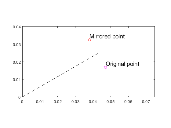
pout_counterclockwise = pout_clockwise.mirror( 2*pi/dimensions.Qr );

Like stated in the documentation, this method mirrors the point around the center of the segment with a width of 2*pi/dimensions.Qr radians. For reference, let's plot both the original point and the mirrored one, and the segment centerline:

clf; hold on; box on;
set(gca, 'XLim', [0 dimensions.Rout*1.5]); daspect([1 1 1]);
pout_clockwise.plot('Original point', 'mo'); %plot after rotation
pout_counterclockwise.plot('Mirrored point', 'ro');

plot([0 dimensions.Rout*cos(pi/dimensions.Qr)], [0 dimensions.Rout*sin(pi/dimensions.Qr)], 'k--');

Creating the tooth body and rotor core

Next, let's create the points for the tooth bottom, and the rotor core.

r_in = dimensions.Rout - dimensions.h_tooth_r; %radial coordinate of tooth bottom

pin_clockwise = Point([sqrt(r_in^2-(dimensions.w_tooth_r_in/2)^2), ...
    -dimensions.w_tooth_r_in/2], 5e-3).rotate( pi/dimensions.Qr );
pin_counterclockwise = pin_clockwise.mirror( 2*pi/dimensions.Qr );

p_core_cw = Point( [r_in, 0], 10e-3);
p_core_ccw = p_core_cw.mirror( 2*pi/dimensions.Qr );

Finally, let's create a Surface object.

O = Point([0,0], 10e-3);

s_core = Surface('core', ...
    geo.line, O, p_core_cw, 'n_cw', ...
    geo.arc, p_core_cw, O, pin_clockwise, ...
    geo.line, pin_clockwise, pout_clockwise, ...
    geo.arc, pout_clockwise, O, pout_counterclockwise, 'n_ag', ...
    geo.line, pout_counterclockwise, pin_counterclockwise, ...
    geo.arc, pin_counterclockwise, O, p_core_ccw, ...
    geo.line, p_core_ccw, O, 'n_ccw');

we set the boundary lines as periodic, to allow mesh replication and periodic boundary conditions:

geo.set_periodic(O, p_core_cw, O, p_core_ccw);

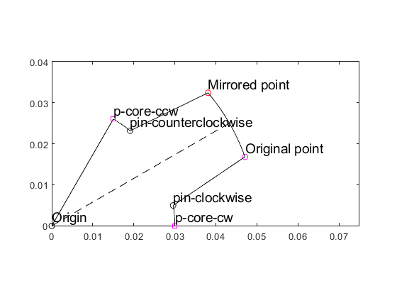
Visualize the surface and points for clarity:

s_core.plot('k');

O.plot('Origin', 'ko');
pin_clockwise.plot('pin-clockwise', 'ko');
pin_counterclockwise.plot('pin-counterclockwise', 'ko');
p_core_cw.plot('p-core-cw', 'ms');
p_core_ccw.plot('p-core-ccw', 'ms');

Now, note that while defining the Surface, we used quite a many named Curves:

n_cw for the clockwise periodic boundary
n_ccw for the counter-clockwise boundary
n_ag for the airgap surface

We'll see later that by defining these Curves, with these exact names, many boring and error-prone tasks can be handled automatically:

replicating a pole or slot segment of a radial-flux machine
setting periodic boundary conditions of analysis
setting up an interface for modelling motion

UPDATE (3.0.1): geo.set_periodic method now does the naming (n_cw, n_ccw) automatically.

Creating a Geometry object

Next, we demonstrate several classes used for creating and analysing finite element models:

GeoBase: a base class for geometry templates.
Material: a class for representing materials
Domain: a class for representing parts of the model geometry.

We begin by first defining some parameters necessary for mesh replication

dimensions.Nrep = 3; %we are not replicating the mesh here
dimensions.sector_angle = 2*pi/dimensions.Qr;

and then initializing the RadialGeometry object:

rotor = RadialGeometry(dimensions) %Geometry objects

rotor = 

  RadialGeometry with properties:

          mesh: []
             p: []
             t: []
         n_dir: []
          n_cw: []
         n_ccw: []
          n_ag: []
         edges: [1×1 struct]
    boundaries: [1×1 struct]
      circuits: []
          data: [1×1 struct]
       domains: []
     materials: []
           PMs: []
          name: ''
    dimensions: [1×1 struct]
        parent: []

As can be seen, the class has quite a few interesting properties like:

p and t : for nodes and triangles respectively, suggesting it is indeed a mesh
materials, domains, circuits, and PMs that we'll take a look at next
n_cw, n_ccw, n_ag, and n_dir that we'll take a brief look on at the end of this tutorial.

Next, we create a Material object for the rotor iron.

Iron = Material.create(4);

Similarly, we create Domain object for representing the rotor core.

Core = Domain('Core', Iron, s_core);

Despite their apparent similarity, Domain objects are entirely different from Surface objects. Indeed, Surface objects

are intended for representing surfaces before meshing
are defined by their boundary alone.

By contrast, Domain objects

consist of meshed surfaces
may consist of one or more Surfaces ...
represent interesting parts of the motor
consist of a single Material
may have a remanence direction (in case of PMs)
may have an orientation (in case of anisotropic materials)
may belong to a Circuit
may contain additional data in domain.data struct

Next, we add the materials and domains to the geometry:

rotor.add_material(Iron);
rotor.add_domain(Core);

Meshing the geometry object

Finally, it is time to mesh the geometry.

rotor.mesh_elementary_geometry();
clf; hold on; box on; axis equal;
rotor.triplot('k');

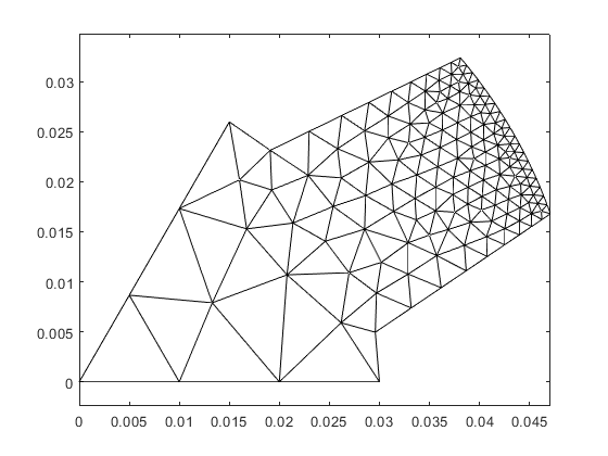
Next, we replicate the mesh to cover the entire symmetry sector:

rotor.replicate_elementary_mesh( )

clf; hold on; box on; axis equal;
rotor.triplot('k');

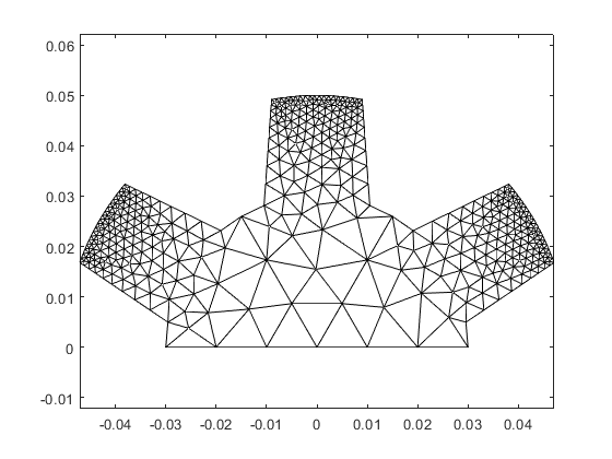
Adding polegap domains

Obviously, our rotor model is not yet complete. Indeed, we need to add some air between the rotor tooth.

This follows exactly the same approach as before, beginning with defining the desired Points and Surfaces.

p_air_cw = Point([dimensions.Rout, 0], 1e-3);
p_air_ccw = p_air_cw.mirror( 2*pi/dimensions.Qr );

s_air_cw = Surface('air', ...
    geo.line, p_core_cw, p_air_cw, 'n_cw', ...
    geo.arc, p_air_cw, O, pout_clockwise, 'n_ag', ...
    geo.line, pout_clockwise, pin_clockwise, ...
    geo.arc, pin_clockwise, O,  p_core_cw);

s_air_ccw = Surface('air', ...
    geo.line, p_core_ccw, p_air_ccw, 'n_ccw', ...
    geo.arc, p_air_ccw, O, pout_counterclockwise, 'n_ag', ...
    geo.line, pout_counterclockwise, pin_counterclockwise, ...
    geo.arc, pin_counterclockwise, O,  p_core_ccw);

geo.set_periodic(p_core_cw, p_air_cw, p_core_ccw, p_air_ccw);

clf; hold on; box on; axis equal;
s_core.plot('k');
s_air_cw.plot('r', 'linewidth',2);
s_air_ccw.plot('r', 'linewidth',2);

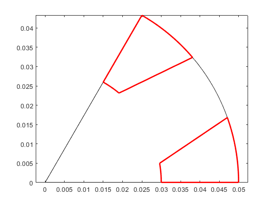
Next, it is turn to add the corresponding new Materials and Domains.

Note that we have to redefine the GeoBase object rotor here, as we can't be adding stuff to an already-meshed geometry.

rotor = RadialGeometry(dimensions);

Air = Material.create(0);
Core = Domain('Core', Iron, s_core);
Polegap = Domain('Polegap', Air, s_air_cw, s_air_ccw);

rotor.add_material(Iron, Air);
rotor.add_domain(Core, Polegap);

Again, we create the elementary mesh...

rotor.mesh_elementary_geometry();
clf; hold on; box on; axis equal;
rotor.triplot('Core', 'k');
rotor.triplot('Polegap', 'r');

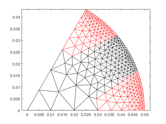
and then replicate it to cover the symmetry sector.

rotor.replicate_elementary_mesh(  )

A Closer look at GeoBase

Earlier, we saw that after meshing the elementary geometry, it was easy to e.g. triplot the Core Domain by referring to its name 'Core'.

Under the hood, this calls, the get_domain method of GeoBase. However, after replicating the elementary mesh, the rotor domain names are a little different:

rotor.domains(1:4).name

ans =

    'Core_1'


ans =

    'Polegap_1'


ans =

    'Core_2'


ans =

    'Polegap_2'

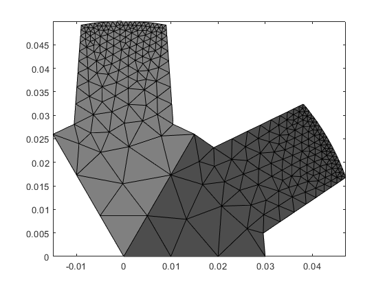
Indeed, each elementary segment of the replicated geometry now has its own Domain. Furthermore, the underscored number at the end of each domain name indicates which replicated sector it belongs to.

clf; hold on; box on; axis equal tight;
rotor.fill('Core_1', [1 1 1]*0.3);
rotor.fill('Core_2', [1 1 1]*0.5);
snapnow

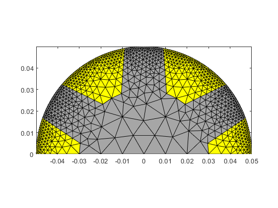
However, thanks to how get_domain is implemented, we can also use the asterisk (*) wildcard character to get all domains corresponding to the original one:

clf; hold on; box on; axis equal tight;
rotor.fill('Core_*', [1 1 1]*0.65);
rotor.fill('Polegap_*', 'y');
snapnow;

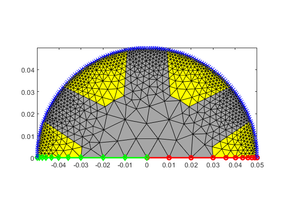
Finally, remember those special Curves we named while defining the Surfaces wayyy back above? Namely:

n_cw for the clockwise periodic boundary
n_ccw for the counter-clockwise boundary
n_ag for the airgap surface
(and n_dir for Dirichlet / flux insulation, had we used any)?

Turns out, we can find the nodes of them all as properties of the Geometry object:

rotor.plot(rotor.n_cw, 'ro-', 'Linewidth', 2);
rotor.plot(rotor.n_ccw, 'gd-', 'Linewidth', 2);
rotor.plot(rotor.n_ag, 'bx-');